Exploratory Data Analysis: Board Game Geek

First I would like to say, welcome to the inaugural post in my Exploratory Data Analysis section.

Typically, EDA is your first venture into a dataset. While you may know general information about the subject matter or have preconceived notions of the features and records, EDA provides us with the chance to discover the intricacies of our data. It also provides us with an understanding on how the values inhabit the data set. (Quote: How do you find a needle in a haystack? You bring a magnet. EDA is said magnet) While a lot of data science savants know techniques used in EDA, when most of us (myself included) actually get our hands on a new dataset the most obvious question is “How and where do I start with EDA?” This is a valid question because EDA doesn’t have a true procedural form. While you might get used to performing the same type of analysis, the nature of EDA involves discovering the unknown or proving that a known is known. I’ve found that the best way to conduct EDA is by:

1. Asking a series of questions about my data.
2. Use EDA techniques to answer my questions.
3. Digest those answers (Think about what I’ve found and what it means).
4. Use those answers to ask new questions or reutilize the older questions.

I don’t know about you, but I love games. Games tend to bring the best and the worse out of everyone. Honestly, playing a game like Monopoly or Settlers of Catan with a group of people and still remaining friends afterwards is like the litmus test of everlasting camaraderie. I like games so much, I started to develop one myself. Elaborating on the game isn’t the real focus of this post but it helps with the question generation of EDA. The game is a super hero vs. super villain card game. Players will get to develop their character further and then play objective based matches. This happens 3 times and depending on the objective described one team (heroes or villains) is declared the winner. I completed a prototype of the game but I was still wondering I could gather insight to intelligently mold the prototype into an official game. Then it clicked “I could use data science to help me in my endeavors”

Materials and Methods

This is where you can find the dataset. It looks like the person who gather this data had the same idea I had only on a much broader scope. Here are a few of the packages I used.

library(tidyverse)
library(corrplot)
library(stringr)

Tidyverse is a godsend for data wrangling. Corrplot is what we will be using to create a correlation matrix, and stringr will help us interact with strings (I use it to “search” or “weed” out specific text and the records related to them)

The process

This dataset was created by another user who is doing something similar but on a much broader scale. Remember a critical function of EDA is to explore your dataset and as a result answer questions. My purpose is: to explore data from similar games in order to gain insight and adapt intelligent design into my own game. That being said, it would be efficient to look at every game available on this dataset, different type of games will require or value different things.

To narrow my efforts I created a subset of data based on a desired feature. That feature being the “mechanics”. In order to hone my search, I thought of the game that most inspired my own Legendary Deck Building Game. One of the foundations of that game, and therefore a foundation of mine was the mechanic of “Deck/ Pool building” where a lot of the interactions with the game are based on creating and drafting cards from the deck. Our dataset also has information that isn’t relevant to my purpose such as the author of the game or it’s URL.

This is what I did to subset the data:

bgg_deck<- bgg %>%
filter(str_detect(mechanic, "Deck / Pool Building")) %>%
select(names, max_time, max_players ,avg_time, year:geek_rating, mechanic, owned, category, weight)

It never hurts to get a general look at summary estimates for your data

summary(bgg_deck)

Now Ive gotten the bulk of the dataset down to the information which can answer my question more efficiently. It’s time to generate some questions

1. Ask a series of question about your data.

The questions can be broad or can be used to help explore your primary function when it comes to what your goals are. Mine is: **to find data from similar games in order to gain insight and adapt intelligent design into my own game. ** so my questions are:

1. Which combination of category appears most with deck pooling
2. What other mechanics are often grouped with this one
3. Which combination of category has the highest rating(Both in Geek and Avg ratings)
4. I want to see the correlation of features among this subset
5. I want to see how the ratings have changed overtime

2. Use EDA to answer those questions.

Question 1.Which combination of category appears most with deck pooling?

Q1 <- bgg_deck %>%
  count(category) %>% # This counts the number of times a particular category is seen
  arrange(desc(n)) %>% # This arranges the number in descending order
  slice(1:10) # This slices the records so that we only get the top 10

Console reads are okay, but let’s see if we can get some visualization out it

g1<-ggplot(data = Q1) +
  geom_bar(aes(x = category, y = n, fill = category), stat = "identity") +
  labs(title = "Top 10 Categories",
       x = "Game Categories",
       y = "# of occurances") +
  theme(axis.ticks = element_blank(), axis.text.x = element_blank())

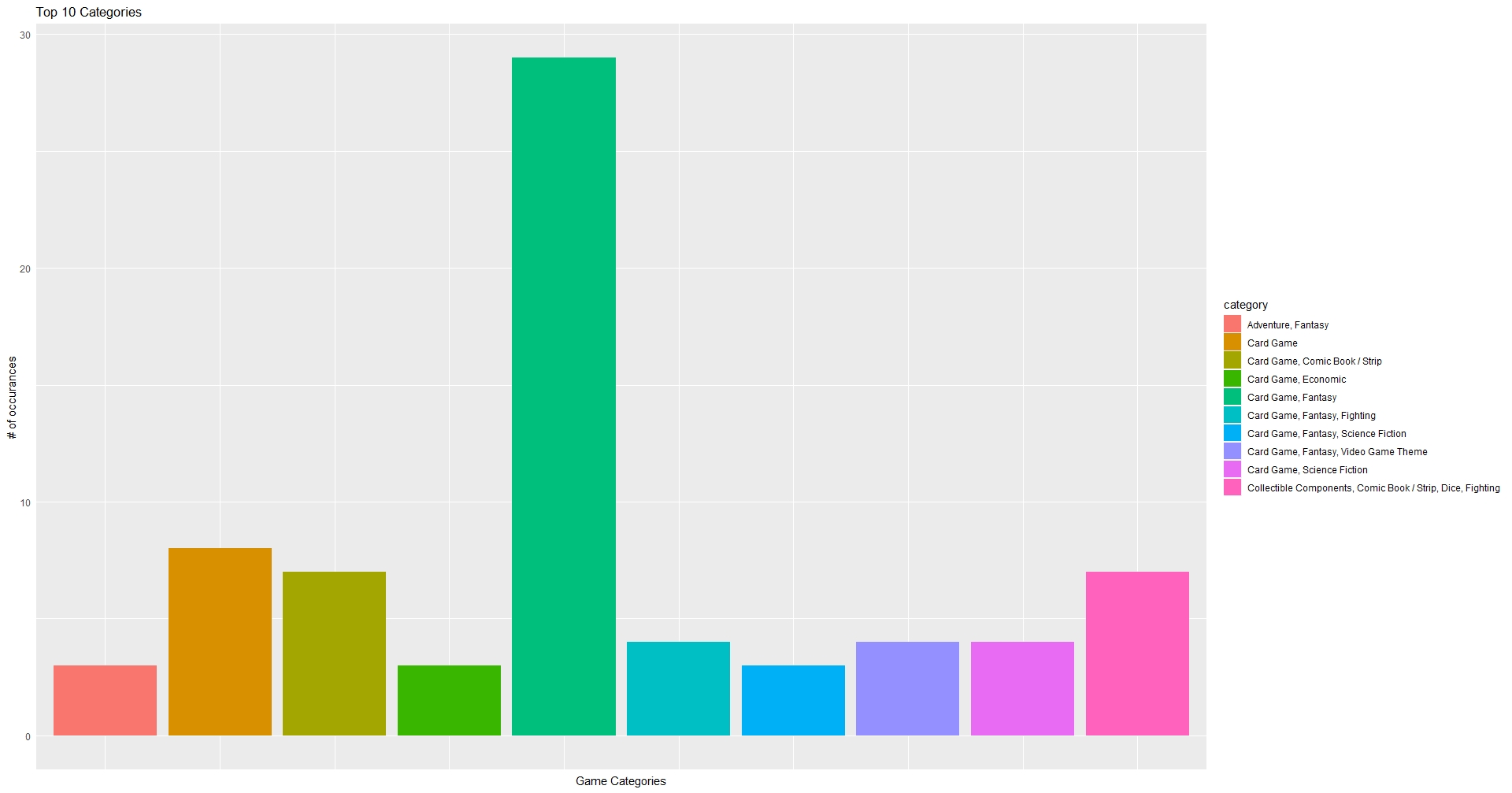You can see that the combination of Comic Book/ Strip appears in the top 5 results. Staggeringly behind the lead result, while modestly ahead of others.

Question 2. What other mechanics are associated with this our target mechanic “Deck / Pool Building”?

Q2 <- bgg_deck %>%
  count(mechanic) %>%
  arrange(desc(n)) %>%
  slice(1:10)
Q2

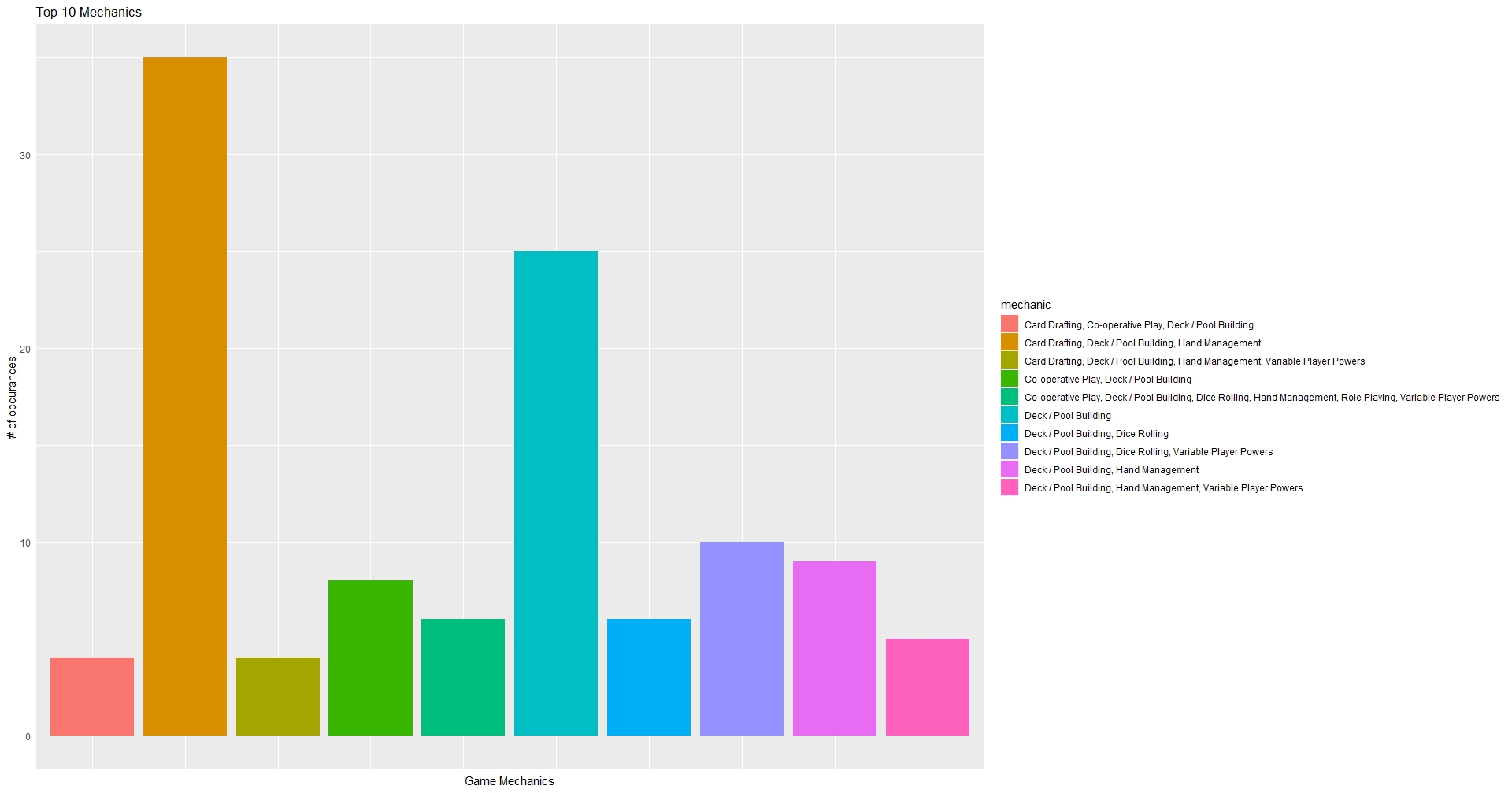
This seems somewhat promising. A large part of my game involves Variable Player Powers mechanics and to a smaller degree Hand Management. Once again we are going to take some time to visualize this.

g2<-ggplot(data = Q2) +
  geom_bar(aes(x = mechanic, y = n, fill = mechanic), stat = "identity") +
  labs(title = "Top 10 Mechanics",
       x = "Game Mechanics",
       y = "# of occurances") +
  theme(axis.ticks = element_blank(), axis.text.x = element_blank())

Question 3. Which combination of category has the highest rating(Both in Geek and Avg ratings)?

This is where I’m starting to put less conjecture and more evidence into my EDA. I want to see which category contains the highest ratings in both Geek and Avg ratings. To clarify, Avg ratings is the average rating of a game generated by the users of Board Game Geek.com. Geek rating is a little bit harder to explain and you can’t see how it is calculated without special privilege. The geek rating is based on the avg rating but it’s used in conjunction with the website’s ranking of games. It was created to prevent manipulation, most noted games with high ratings but low votes climbing the ranking charts. They keep the algorithm a secret so I can’t give you much more information other than that.

# Using Tidy to group and summarize. Shown on the console will be the results of the geek_rating
bgg_deck %>%
group_by(category) %>%
summarize(mean_geek_rating = mean(geek_rating), mean_avg_rating = mean(avg_rating)) %>%
arrange(desc(mean_geek_rating))
# By changing the code a bit, we can see the top mean_avg_rating
bgg_deck %>%
group_by(category) %>%
summarize(mean_geek_rating = mean(geek_rating), mean_avg_rating = mean(avg_rating)) %>%
arrange(desc(mean_avg_rating))

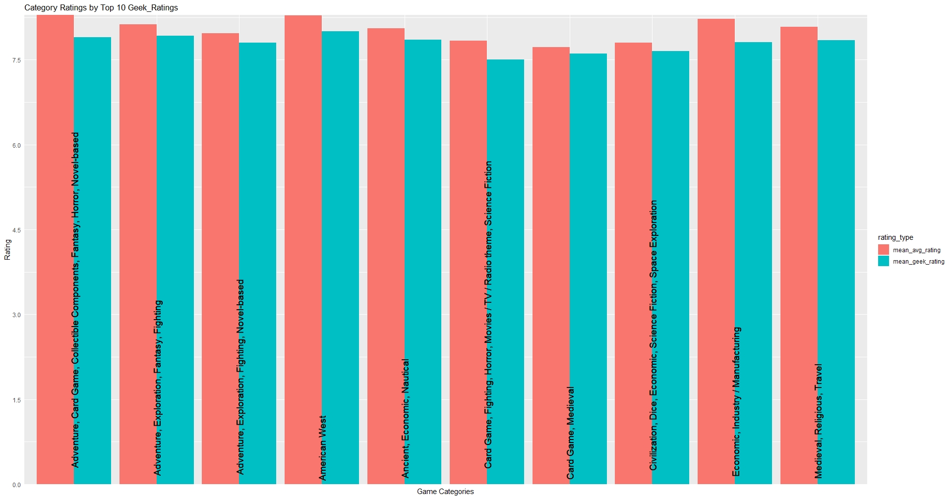
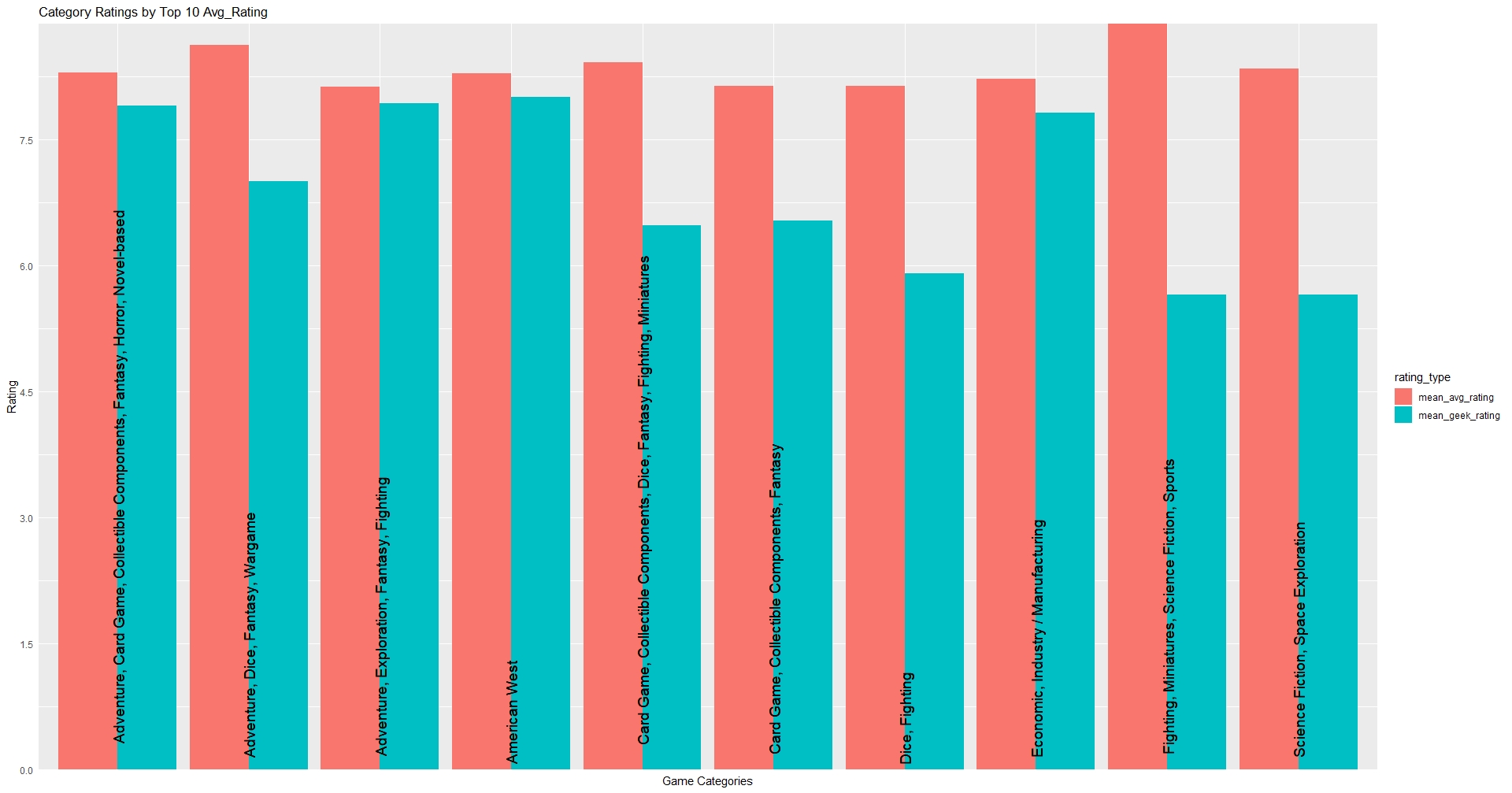
We can see something very interesting. There seems to be a disconnect between the mean_geek_rating and the mean_avg_rating Console reads are nice but lets try to visualize our results. I am also going to backtrack a little in order to introduce another great tool you can utilize from the Tidy package. That tool is called Gather. This Geek_rating

Q3_geek <- bgg_deck %>%
  group_by(category) %>%
  summarize( mean_geek_rating = mean(geek_rating), mean_avg_rating = mean(avg_rating)) %>%
  arrange(desc(mean_geek_rating)) %>% # This arranges by highest to lowest
  slice(1:10) %>% #slice to make it a top 10
  gather("mean_geek_rating","mean_avg_rating", key = "rating_type", value = "rating") 
# The added gather() function will allow us to compare both types of ratings to see how they differ
Q3_geek

Avg_rating

Q3_avg <- bgg_deck %>%
  group_by(category) %>%
  summarize( mean_geek_rating = mean(geek_rating), mean_avg_rating = mean(avg_rating)) %>%
  arrange(desc(mean_avg_rating)) %>%
  slice(1:10) %>%
  gather("mean_geek_rating","mean_avg_rating", key = "rating_type", value = "rating")
Q3_avg

Now let us visualize the data: Highest geek_rating

g3g<-ggplot(data = Q3_geek) +
  geom_bar(aes(x = category, y = rating, fill = rating_type),position = "dodge", stat = "identity") +
  geom_text(aes(y = 0, x = category, label = category), data = Q3_geek, angle = 90, hjust = -.05, size = 5 ) +
  scale_y_continuous(breaks = seq(0, 10, by = 1.5), expand = c(0,0)) +
  labs(title = paste("Category Ratings by Top 10 Geek_Ratings"),
       x = "Game Categories",
       y = "Rating") +
  theme(axis.ticks = element_blank(), axis.text.x = element_blank())
g3g

Highest avg_rating

g3a<-ggplot(data = Q3_avg) +
  geom_bar(aes(x = category, y = rating, fill = rating_type),position = "dodge", stat = "identity") +
  geom_text(aes(y = 0, x = category, label = category), data = Q3_avg, angle = 90, hjust = -.05, size = 5 ) +
  scale_y_continuous(breaks = seq(0, 10, by = 1.5), expand = c(0,0)) +
  labs(title = paste("Category Ratings by Top 10 Avg_Rating"),
       x = "Game Categories",
       y = "Rating") +
  theme(axis.ticks = element_blank(), axis.text.x = element_blank())

Question 4. What is the correlation of features among this subset?

Now I am going to create a correlation matrix and then correlation plot to visualize.

bgg_deck_corr <-bgg_deck %>%
  select(max_time:geek_rating,owned,weight) # This time I am removing non-numerical features from the dataset
bgg_deck_corr <-round(cor(bgg_deck_corr), 2) # This turns our data into the matrix required

I created a new object leaving only the numerical features I felt interested in. The last line of code will convert our data into a correlation matrix. Next lets visualize.

corrplot(bgg_deck_corr, method = "color", insig = "blank",
         order = "hclust", # performs the clustering, which makes the graph much easier to digest
         addCoef.col = "black"
)

Question 5. I want to see how the ratings have changed overtime?

Remember we have two different types of ratings. Instead of creating two separate graphs, we can actually use a facet wrap to display both types of ratings within the same graph.

First lets revisit the code we created when we used the gather() function but with a few amendments.

bgg_deck_TS<- bgg_deck %>%
  group_by( year) %>%
  summarize( mean_geek_rating = mean(geek_rating), mean_avg_rating = mean(avg_rating)) %>%
  gather("mean_geek_rating","mean_avg_rating", key = "rating_type", value = "rating")
bgg_deck_TS

Notice I removed the slice() and arrange() because those don’t matter to me anymore. I’ve also replaced “category” with the “year” feature into my group_by() Okay lets visualize this:

ggplot(data = bgg_deck_TS) +
  geom_line(aes(x = year, y = rating, color = rating_type, group = rating_type)) +
  facet_wrap(~ rating_type) + # Facet_wrap will allow me to display additional variables.
  labs(title = paste("Ratings Throught the Years"),
       x = "Years",
       y = "Rating") +
  theme_classic()

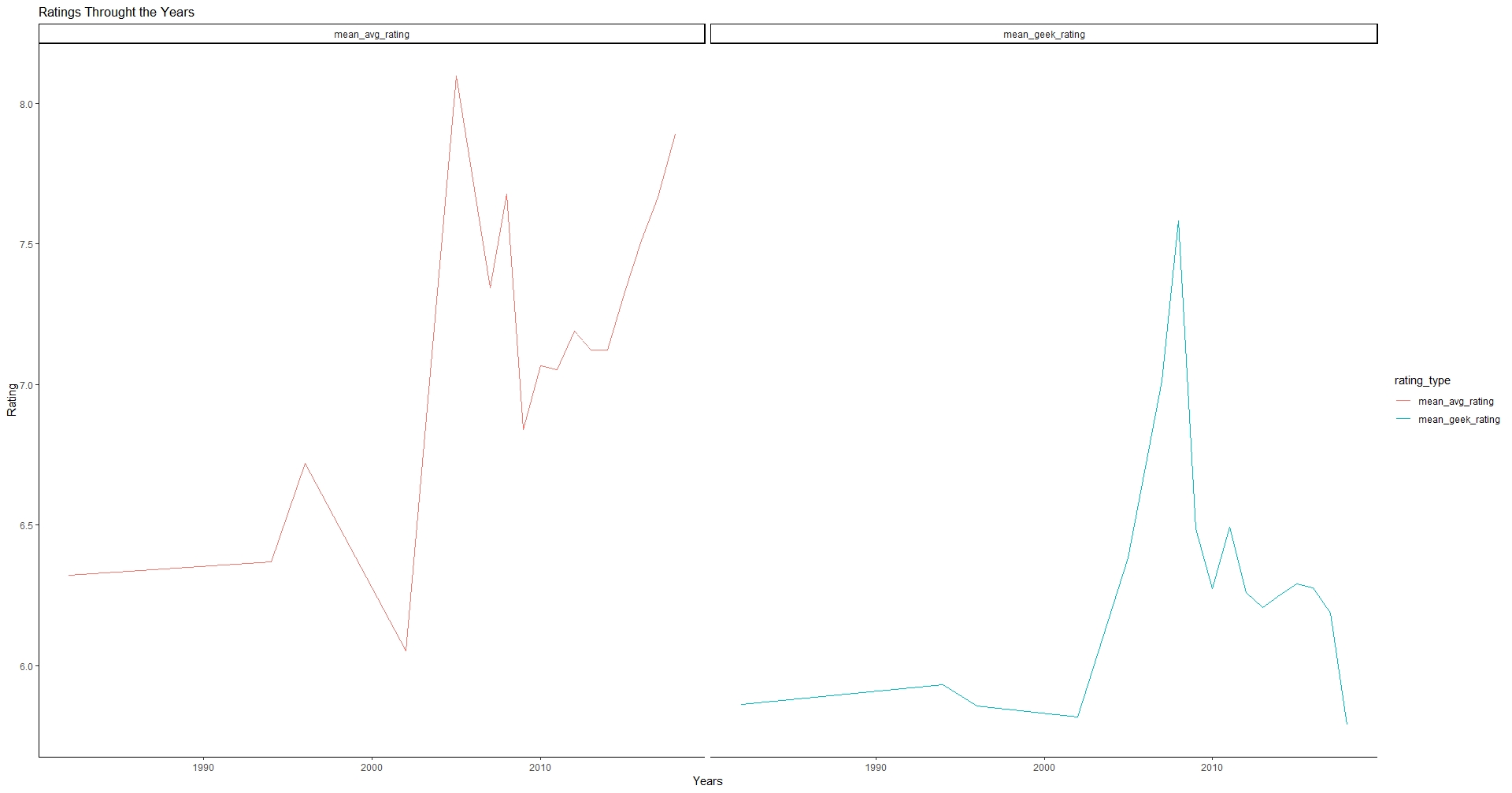
Here we can see that from the mean_avg_rating, ratings have been climbing upwards, however in the mean_geek_rating feature, ratings have actually been declining.

3. Digest those answers

Insight gained from questions 1 and 2

As stated earlier my purpose was : to explore data from similar games in order to gain insight and adapt intelligent design into my own game. The insight I gained from my first questions were used to help me see if the themes and mechanics of my own game appear. The results of those seem fairly promising. If I had to lump my game prototype into a category it would be “Deck/Pool Building, Hand Management, Variables Player Powers”. While this does make it into the top 10, it is at the bottom of the list. Why is that? Maybe the combination doesn’t work too well?

The Combination of category I would place the prototype in would be Card Game, Comic Book/Strip which is the 3rd most occurring in the Top 10.

Insight gained from question 3 and 4

Since I don’t have any record of how financially successful these game are the metric for success I decided to use was the ratings. Since there are two types of ratings I decided to make two graphs, one indicating the mean_avg_rating and the other contains the mean_geek_ratings of a particular category of games. This means I’m assuming the higher the rating the more successful the game. The category I placed my prototype in doesn’t make the top 10. What is more interesting is the difference between the ratings when we are looking at the top 10 highest. While mean_geek_rating contains similar records among geek_rating and avg_rating, The top 10 avg_ratings shows a significant disconnect between the two ratings.

When we look at the correlation graph, again I am using the geek and avg ratings as a metric for success. My goal is to see if another feature within the dataset has a positive or negative correlation with either of these. Following this, I could reduce or increase those features in my prototype. Unfortunately I didn’t find any strong correlation from the rating features in which I could manipulate while developing my prototype. The strongest of those is “owned” which I have no direct control over. This correlation matrix does provide something really valuable, which I will discuss in the last part of EDA

Insight gained from questions 5

This shows me that over the years, games that contain the “Deck/ Pool Building” mechanic have been rising in terms of their mean_avg_rating while decreasing in terms of their mean_geek_rating. If I saw a steady decrease in both, I might make the decision to ditch the project or investigate meaning behind the decline.

4. Use those answers to ask new questions or reutilize the older questions

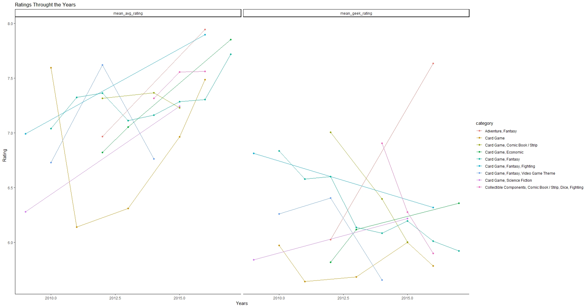
I can use these answers to further explore my data. For instance, what if I explored the feature weight? I could see how the complexity of a game fits with its category or mechanic. I spent a lot of time looking at game mechanics and categories. Later on I started using the ratings as a metric for success. Why not combine them?

#In this part, I am establishing our new group based on the results from our "Q1"
Q1
bgg_deck_TS2<- bgg_deck %>%
  group_by(year, category) %>%
  filter(category %in% c("Card Game", "Card Game, Fantasy","Card Game, Comic Book / Strip","Collectible Components, Comic Book / Strip, Dice, Fighting",
                         "Card Game, Fantasy, Fighting","Card Game, Fantasy, Video Game Theme", "Card Game, Science Fiction", "Adventure, Fantasy",
                         "Card Game, Economic","Card Game, Fantasy, Science Fiction ")) %>%
  summarize( mean_geek_rating = mean(geek_rating), mean_avg_rating = mean(avg_rating)) %>%
  gather("mean_geek_rating","mean_avg_rating", key = "rating_type", value = "rating")
bgg_deck_TS2
# Next I'll create a graph
ggplot(data = bgg_deck_TS2) +
  geom_line(aes(x = year, y = rating, color = category)) +
  geom_point(aes(x = year, y = rating, color = category))+
  facet_wrap(~ rating_type) +
  labs(title = paste("Ratings Throught the Years"),
       x = "Years",
       y = "Rating") +
  theme_classic()

Conclusion

The moment most of us were waiting for. This concludes my exploration in EDA. I hope you found this informative, I hope this gave you a better understand on how to apply EDA to your own projects. Finally I hope you all come back to learn more.